st_kde

suppressWarnings(library(SfSpHelpers))
suppressWarnings(library(raster))
#> Loading required package: sp
suppressWarnings(library(sf))
#> Linking to GEOS 3.10.2, GDAL 3.4.1, PROJ 8.2.1; sf_use_s2() is TRUE
suppressWarnings(library(magrittr))
#> 
#> Attaching package: 'magrittr'
#> The following object is masked from 'package:raster':
#> 
#>     extract
suppressWarnings(library(dplyr))
#> 
#> Attaching package: 'dplyr'
#> The following objects are masked from 'package:raster':
#> 
#>     intersect, select, union
#> The following objects are masked from 'package:stats':
#> 
#>     filter, lag
#> The following objects are masked from 'package:base':
#> 
#>     intersect, setdiff, setequal, union
suppressWarnings(library(ggplot2))
suppressWarnings(library(RColorBrewer))

Data

  #Trees
  shp_trees <-  st_read('https://www.donneesquebec.ca/recherche/dataset/bc5afddf-9439-4e96-84fb-f91847b722be/resource/bbdca0dd-82df-42f9-845b-32348debf8ab/download/vdq-arbrepotentielremarquable.geojson')
#> Reading layer `D:/fmeserver2017///resources/data/\DO\PUBLICATION\vdq-arbrepotentielremarquable.geojson' from data source `https://www.donneesquebec.ca/recherche/dataset/bc5afddf-9439-4e96-84fb-f91847b722be/resource/bbdca0dd-82df-42f9-845b-32348debf8ab/download/vdq-arbrepotentielremarquable.geojson' 
#>   using driver `GeoJSON'
#> Simple feature collection with 707 features and 11 fields
#> Geometry type: POINT
#> Dimension:     XY
#> Bounding box:  xmin: -71.41288 ymin: 46.73784 xmax: -71.15738 ymax: 46.93477
#> Geodetic CRS:  WGS 84
 
  #Neighborhoods
  shp_neigh <-  get_zipped_remote_shapefile("https://www.donneesquebec.ca/recherche/dataset/5b1ae6f2-6719-46df-bd2f-e57a7034c917/resource/508594dc-b090-407c-9489-73a1b46a8477/download/vdq-quartier.zip")
#> [1] "Downloading to tmp directory"
#> Reading layer `vdq-quartier' from data source `/tmp/RtmpW5XkwL' using driver `ESRI Shapefile'
#> Simple feature collection with 35 features and 4 fields
#> Geometry type: MULTIPOLYGON
#> Dimension:     XYZ
#> Bounding box:  xmin: -71.54908 ymin: 46.73355 xmax: -71.13833 ymax: 46.98074
#> z_range:       zmin: 0 zmax: 0
#> Geodetic CRS:  WGS 84

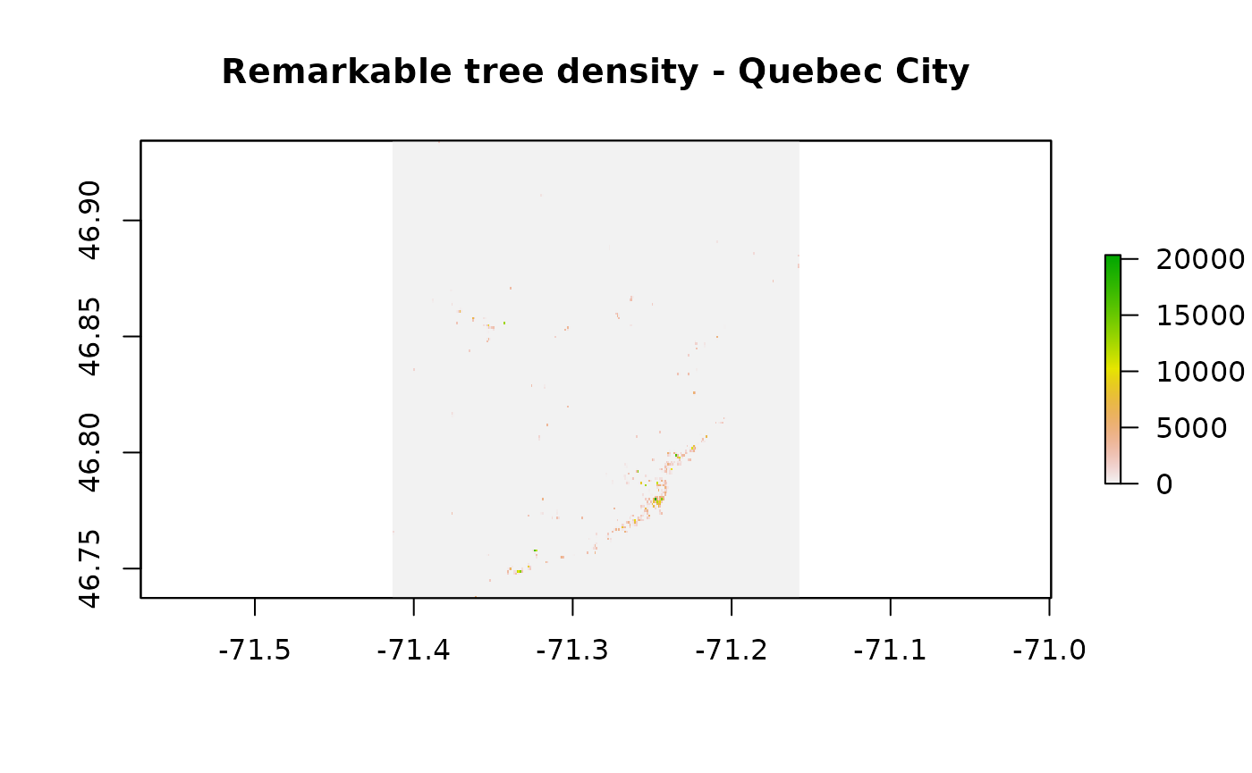
2D raster KDE plot - default

  rasterKDECentroids <- st_kde(shp_trees , cellsize = 0.001, bandwith =c(.001, .001 ) )
  plot(rasterKDECentroids$layer, main='Remarkable tree density - Quebec City')

GGplot version

  df_rast <- rasterKDECentroids$layer %>% as.data.frame(xy=T)
  
  if(! ('NOM' %in% colnames(shp_neigh))){
    knitr::knit_exit()
  }
  extended_cols <- colorRampPalette(brewer.pal(8, "Set3"))(n_distinct(shp_neigh[['NOM']]))
  
  ggplot() + 
    geom_tile(data=df_rast, aes(x=x,y=y,fill=layer),alpha=0.2) + 
    geom_sf(data=shp_neigh, aes(col=NOM),alpha=0) + 
    scale_fill_viridis_c() + 
    scale_color_manual(values = extended_cols) + 
    ggplot2::theme_dark(base_family="Roboto Condensed", base_size=11.5) +
    guides( color = "none") 

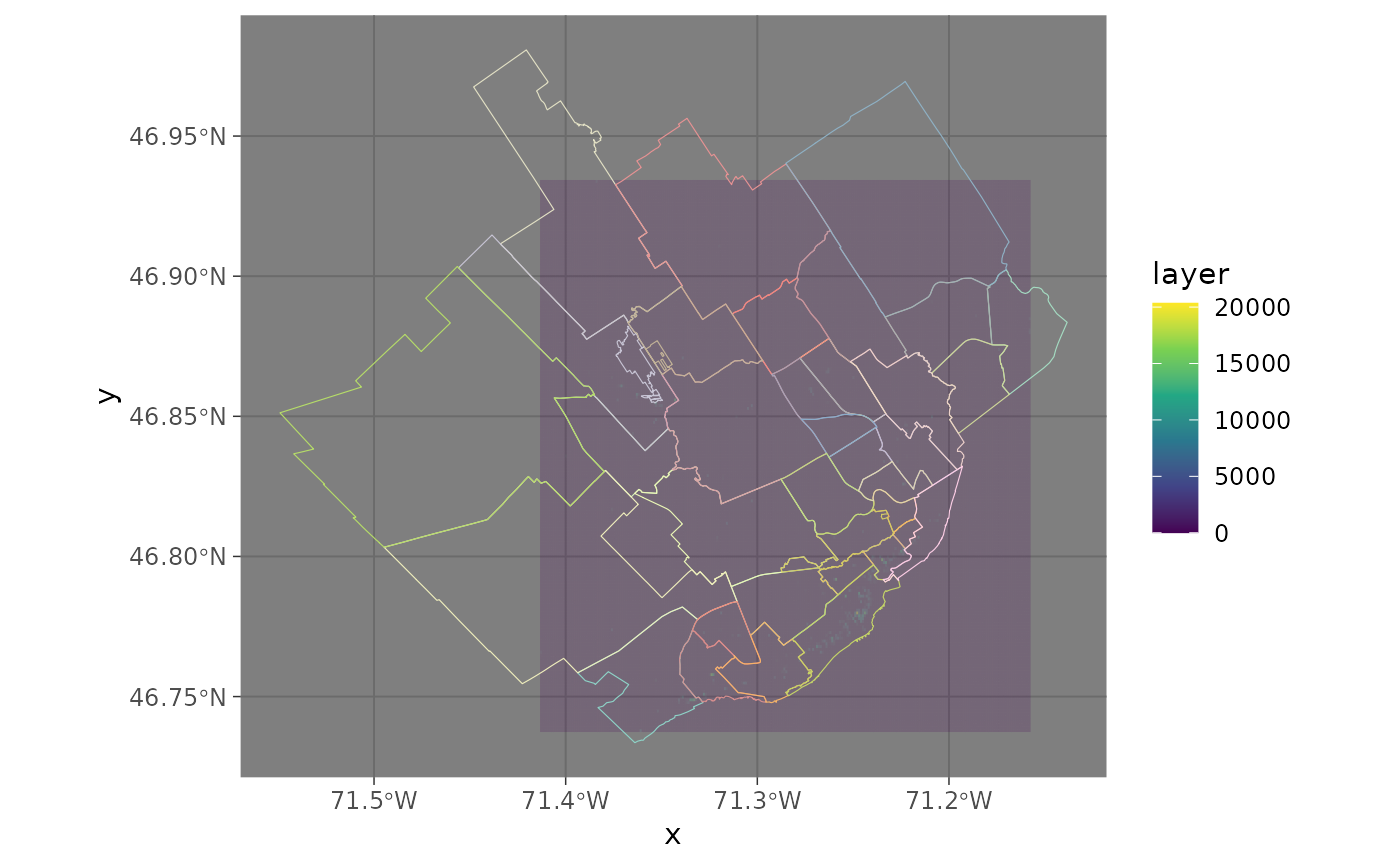
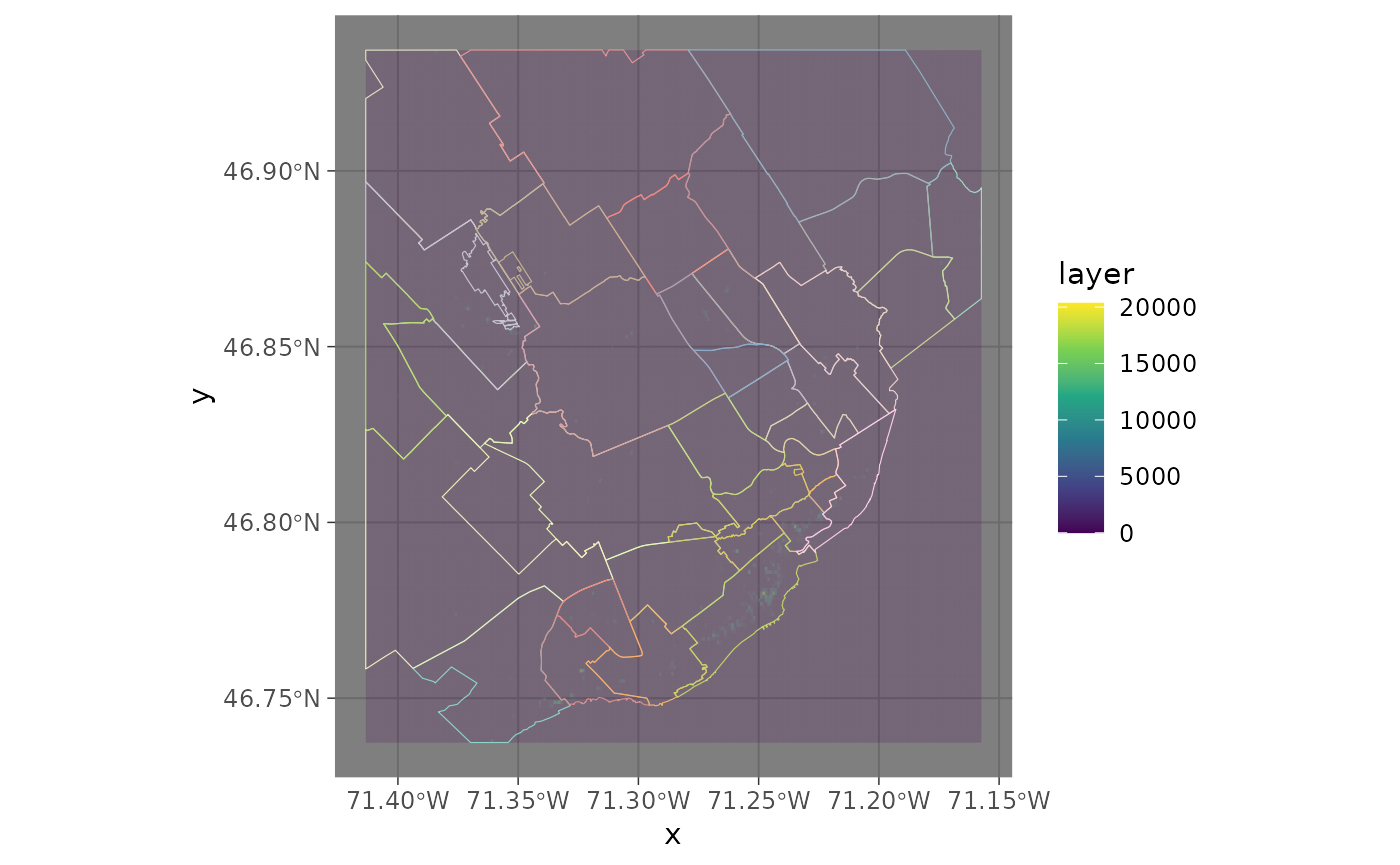
Zoom in using functions in bbox

shp_bbox_raster <- bbox_from_vector( extent(rasterKDECentroids) , crs=4326)

shp_neigh_filtered <- st_intersection(shp_neigh %>% st_zm(),
                                      shp_bbox_raster)
#> Warning: attribute variables are assumed to be spatially constant throughout all
#> geometries

  ggplot() + 
    geom_tile(data=df_rast, aes(x=x,y=y,fill=layer),alpha=0.2) + 
    geom_sf(data=shp_neigh_filtered, aes(col=NOM),alpha=0) + 
    scale_fill_viridis_c() + 
    scale_color_manual(values = extended_cols) + 
    ggplot2::theme_dark(base_family="Roboto Condensed", base_size=11.5) +
    guides( color = 'none') 

Polygon contours

  #get_polygon_heatmap Works with polygons also (takes centroid implicitely)
  shp_polyons <- get_polygon_heatmap(shp_trees , bw=.001, gsize=500 )
#> Warning in st_centroid.sf(shp): st_centroid assumes attributes are constant over
#> geometries of x
#> Warning: The `x` argument of `as_tibble.matrix()` must have unique column names if
#> `.name_repair` is omitted as of tibble 2.0.0.
#> ℹ Using compatibility `.name_repair`.
#> ℹ The deprecated feature was likely used in the SfSpHelpers package.
#>   Please report the issue to the authors.
 
 
#Can use the colors produced automatically, but this is a red to yellow gradient 
ggplot(shp_polyons)+
    geom_sf(aes( fill = colors),lwd=0) +
    scale_fill_identity() +
    geom_sf(data=shp_neigh, aes(col=NOM),alpha=0) + 
    ggplot2::theme_minimal(base_family="Roboto Condensed", base_size=11.5) +
    guides( color = 'none') 

 
#Can simply use viridis discrete
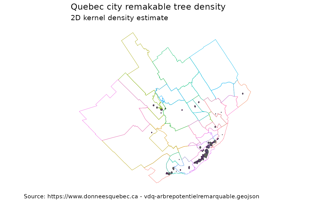
ggplot(shp_polyons)+
  geom_sf( aes(fill=colors) ,lwd=0) +
  geom_sf(data=shp_neigh, aes(col=NOM),alpha=0) + 
  scale_fill_viridis_d()+
  coord_sf(datum = NA) + 
  ggplot2::theme_minimal(base_family="Roboto Condensed", base_size=11.5) +
  guides( color = 'none', fill = 'none') +
  ggtitle("Quebec city remakable tree density") + 
  labs(subtitle = "2D kernel density estimate",
         caption ='Source: https://www.donneesquebec.ca - vdq-arbrepotentielremarquable.geojson')

ggsave('tree_kde.png', width = 7, height = 7)